The FTLinefitter tool runs under IDL 8.7 (full version or Virtual Machine), and is available as a [.SAV file] of the compiled routines or a [full installation] including a Runtime version of IDL. (Version 1.93 Last modified Oct 29 2019).
Changes in version 1.93:
- Compiled for IDL 8.7.
- Added covariance matrix to FTFitter object parameters
Changes in version 1.92:
- Support for revised SPIRE FITS format files.
- Fixed bug in cube coordinate parsing.
- Option to show\hide continuum.
- Line names in table can be changed. Duplicate names are allowed, but may cause unforeseen problems with the plot object.
- FTS-2 FITS file support.
- Fixed bugs with trimming and limit values.
Changes in version 1.9:
- Recompiled for IDL 8.2
- Additional SPIRE FITS file format support
Changes in version 1.8:
- added support for SpectralSimpleCube FITS files
- added support for reading IDL .sav files
- added option to read in error spectrum
Known issues:
- When the spectral intensity is small (e.g. 10^-16) the returned error estimates will likely not be valid
Download the archive and extract to a folder of your choosing. The archive includes the main code in FTFitter_gui.sav, a subfolder named 'docs' which contains the documentation, and a subfolder named 'data' which contains the line parameter XML schema definition.
If you are using the full VM distribution, just unzip and run the FTFITTER_GUI.exe file.
If using a full licensed version of IDL, you can include the installation folder in your IDL search path or manually load the code by typing: restore,'pathname' , where pathname is the fully qualified path to FTFitter_gui.sav. Typing ftfitter_gui in the command line will launch the GUI. When starting, the GUI searches for a settings file named 'FTFITTER_GUI_settings.sav' in the current directory. If this file is not found, default settings will be used -so be careful to set reasonable values for all parameters before attempting a fit. Upon exit, the GUI will store the current program parameters to the FTFITTER_GUI_settings.sav file.
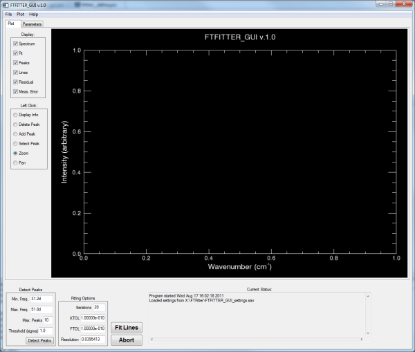
The main screen of the FTFitter GUI is shown below.
- There is a Plot tab for displaying the current lines, spectrum, and model, and a Parameters tab which provides a table for viewing and editing individual line parameters.
- The 'Display' checkboxes determine which features are shown in the interactive plot.
- The 'Left Click' radio buttons determine what occurs when the left mouse button is used in the plot window.
- 'Zoom' allows a zoom window to be used while clicking and dragging the mouse. Right clicking restores the previous zoom. The scroll wheel can also be used to zoom in or out on the current mouse location.
- 'Select Peak' selects the clicked peak in the parameter table.
- The fields in the 'Detect Peaks' box set the options for the automatic peak detection algorithm. When the 'Detect Peaks' button is pressed, the algorithm looks for peaks in the residual spectrum with amplitude higher than the specified threshold above the mean, up to a maximum number of peaks. It is usually best to detect small numbers of peaks at a time, and then perform a fit before detecting more peaks.
- The 'Fitting Options' fields define the maximum number of iterations and the tolerances for the convergence criteria.
- Iterations defines the maximum number of iterations to perform. It is usually best to keep this number small.
- XTOL measures the relative error desired in the approximate solution. The default is 1e-10.
- FTOL measures the relative error desired in the sum of squares. The default is 1e-10.
- Resolution is the true resolution of the spectrum, not including any zeropadding. This defines the linewidth of the unresolved lineshapes.
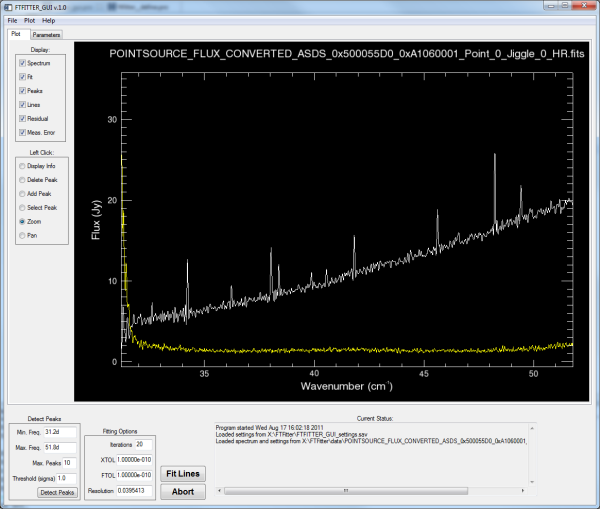
Before using any other features, a spectrum must be loaded. FTFitter_GUI currently supports Herschel SPIRE FITS files and GRAMS compatible SPC files. The image below shows a SPIRE spectrum and associated error spectrum in yellow. The error spectrum is used to define the weighting of each data point during the fit. If the error spectrum is zero, then uniform weighting will be used but the uncertainties in the retrieved parameters will not be meaningful.
Once a spectrum is loaded, parameters can be loaded from compatible XML files using the File menu. Note that the XML files should be placed in the 'data' subdirectory, or else the 'ftfitter_line_parameters.xsd' schema file will need to be placed in the same directory as the parameter file.
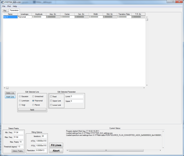
Alternatively, the Parameters Tab can be used to view and edit line parameters. In the image below, a Polynomial baseline has been added by selecting the Polynomial radio button and clicking 'Insert Line'. Nate that when a cell is selected in the table, the column labels change according to the lineshape that is currently selected.
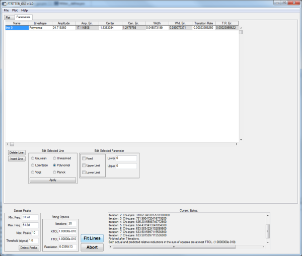
Now that the polynomial baseline is defined, a quick fit to the data can be performed by clicking the 'Fit Lines' button. The image below shows the result of the fit; the optimized polynomial coefficients are shown in the table, and the status window shows the results of each iteration and the condition that triggered the end of the fitting process.
By switching to the Plot Tab, the model spectrum can be seen in green, and the residual error in light blue (as shown below). Note that the measured error trace has been hidden by deselecting the 'Meas. Error' display checbox.
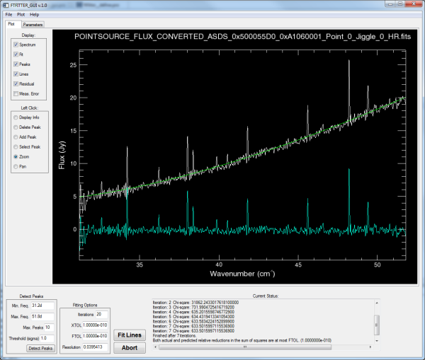
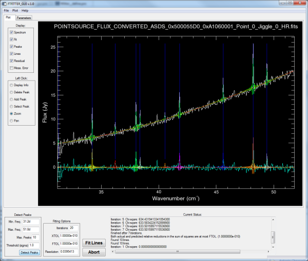
The automatic peak detection feature can now be used to identify local maxima in the spectrum that are larger than the threshold parameter from the mean, between the minimum and maximum frequencies. The image below shows the result of finding 10 peaks in the residual spectrum over the full range. Peak locations are shown as blue lines (which can be hidden using the 'Peaks' checkbox), and the individual lineshapes are shown in random colors (which can be hidden using the 'Lines' checkbox). The model spectrum in green has beed updated to include the continuum and the lines. The default to use unresolved lineshapes for the automatically detected lines.
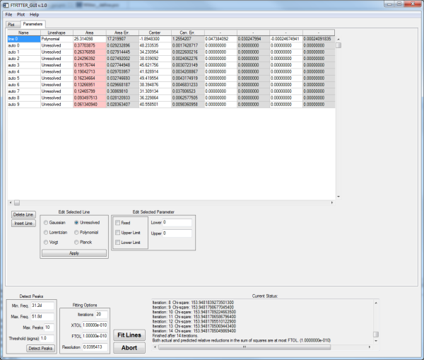
Switching to the Parameters Tab shows the newly added lines. The uncertainties in the parameters are shown in the Err columns. Cells are color-coded with the following scheme:
- White - editable field
- Grey - non-editable field (e.g. the uncertainty values)
- Pink - parameter has at least one limit defined
- Red - parameter value is pegged at a limit
- Light Blue - the parameter is fixed
- Yellow - the parameter uncertainty is suspiciously large
The lineshape for a line or multiple lines can be changed by selecting the line, chosing a new lineshape button, and hitting 'Apply'. Parameter values can be changed by typing directly into the cell. Note that columns that are not relevant to the currently selected lineshape are labeled with '-'. Any values in these cells will not be considered in calculating those lineshapes.
In the image below, all 10 automatically detected peaks have been selected, and their lineshapes have been changed to Gaussian.
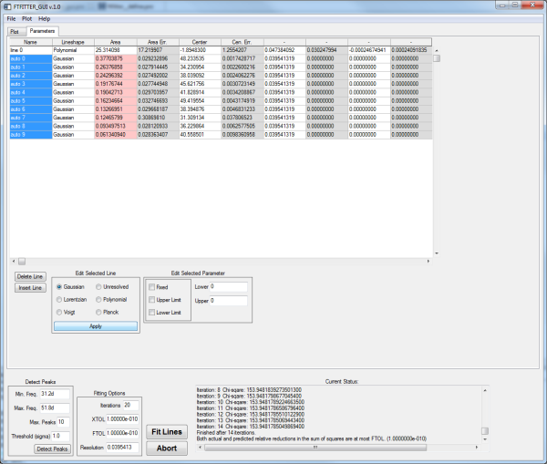
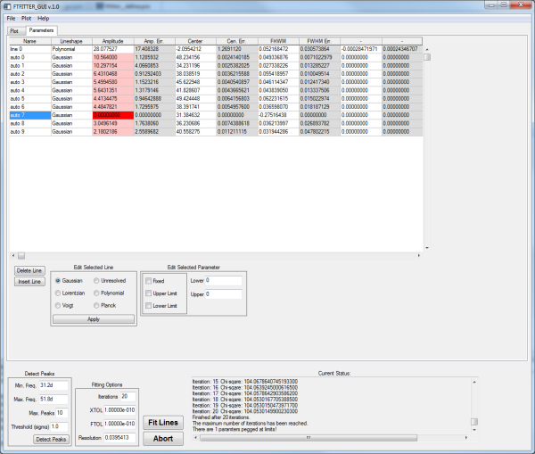
The Gaussian lines can now be fit by clicking the 'Fit Lines' button. The result is shown below. Note that the status window indicates that the fit did not converge, and there is one parameter pegged at a limit. The table cell highlighted in red shows the invalid parameter. This lineshape has been reduced to zero amplitude and its FWHM is not meaningful. The line can be altered manually or deleted before running the fit again.
The line parameters can be saved as an XML file for future use by using the File menu.
If you want to use the FTFitter object in your own script, you must first restore the .sav file into your IDL session. You can then create an FTFitter object and call the methods according to the documentation provided in 'FTFitter_Object_Documentation.pdf'.
